2015-04-29

Dr Foreman-Mackey

It was a great day at CampHogg today! Foreman-Mackey defended his PhD thesis with a great talk. Although his thesis also contained chapters about MCMC sampling, exoplanet populations, and finding isolated transit events in lightcurves, he concentrated his oral presentation on the discovery of periodic transits in the K2 data. This permitted him to touch on many aspects of his work, including especially the marginalization out of systematics (instrument-induced signals). He made a very strong case that we need to fit the systematics simultaneously with the signals of interest, because in any other approach (any pre-filtering or data conditioning method), you end up either very strongly restricting the systematics model (so it doesn't do what you need) or else you end up over-fitting and distorting your transit signals. The thesis talk was followed by extensive questioning and the signing of forms.

As my loyal reader can infer from what's written in the many posts on this blog, Foreman-Mackey has had a huge impact on every aspect of my scientific life. I have learned far more from him than he has learned from me. He has achieved a lot, in tool building and in the production of valuable scientific results. I still get a few more weeks of Foreman-Mackey but then he is off to Seattle to start his Sagan Fellowship.

2015-04-28

#astrohackny, APOGEE, chaos, brown dwarfs

At #astrohackny, Ben Weaver showed us more development he has done on fitting the individual-exposure radial velocities in the APOGEE data. It looks to me very likely that he will be able to improve the APOGEE data analysis with these, and maybe also discover some cool things.

After the hacking, I spent time with Price-Whelan and Johnston talking about chaos. I admitted that I have no idea what constitutes a chaotic orbit! There are differences, it appears, between diffusion in frequency space and Lyapunov times; these aren't in contradiction, exactly, but the differences are surprising given my (trivial, incomplete) intuition. Something is odd to me about the related but seemingly very different points that a chaotic orbit is 5-space-filling (not just 3-torus-filling) and that it has a positive Lyapunov exponent and that it diffuses in frequency space. These all seem like three very different manifestations of chaos.

Kopytova and I spoke about fitting brown-dwarf spectra. We identified a set of easy projects, one of which is to fit the spectral data with a flexible calibration (or, equivalently, continuum) model. For the longer term, we talked about making data-driven improvements to the models, which seem to be incomplete or in need of work in the H band.

2015-04-27

are GRBs beamed?

It was all GRBs today, with Maryam Modjaz (NYU) at coffee talking about this paper that finds a gamma-ray burst by its optical emission (that is, not by having a gamma-ray or x-ray trigger). Then at lunch, more GRBs with Modjaz talking about the GRB progenitors, about which we only have indirect information from looking at environments (and especially abundances). I asked my usual questions about beaming: We know from models of the emission that GRBs should be highly beamed, and that the optical should be much less beamed than the gamma-rays. But that means that there must be many GRB-like optical transients that don't have gamma-ray counterparts. None have been found! What gives? In general, the empirical evidence for beaming in astrophysical sources has always been weak (think of all the arguments about quasar unification), with pulsars an exception. Of course the detailed answers to this question involve the relative brightnesses, time scales, and spectral energy distributions of the way-off-axis emisssion, so there is quite a bit of theory to do to interpret the observations, but right now it is looking hard to reconcile all the theory and observations around GRB beaming.

2015-04-26

super-Nyquist writing and plotting

I got some quality research time in on the weekend. I put words into the document that explains the variable-exposure-time results, including for sensitivity to, statistical independence among, and recovery of harmonic signals in time-series data. Also related to this I worked on the plotting of the results. If you are going to frequencies way above the Nyquist frequency, you have to use a huge frequency grid, if you want to resolve the modes!

2015-04-24

self-calibration of GALEX, regularizing a PSF model

At group meeting, Dun Wang showed his first results from his work on the GALEX photons. He showed some example data from a scan across the Galactic plane and back, performed by Schiminovich in the spacecraft's last days. The naively built image has a double point-spread function, because the satellite attitude file is not quite right. Wang then showed that on second (or even half-second) time scales, he can infer the pointing, either by cross-correlating images, or else correlating with known stars. So the satellite pointing could be very well calibrated with a data-driven model. That's awesome!

Also at group meeting, Vakili discussed taking his model of the point-spread function up to super-resolution (that is, modeling the PSF at a resolution higher than the imaging data with which we constrain it). The model is super-degenerate, so we are in the process of adding (willy nilly) lots of different regularizations. My "big idea" at the meeting was to model the PSF using only smooth functions, because we know (for very deep physical reasons) that the PSF cannot have features or structure below some fundamental angular scale (set by the diameter of the telescope aperture!).

2015-04-23

aliasing and orthogonality

I worked on computing cosine distances (dot products) between different frequencies as they would appear in a data set with uniform time spacing and uniform exposure time, as compared to a similar data set but with non-uniform time spacing and exposure times. In the uniform case, the different frequencies are exactly orthogonal (that is the magic of the Fourier transform) but there are also exact aliases among frequencies above the Nyquist limit. That is, for every frequency there are many aliases at very high frequencies. In the non-uniform case, all of these aliases disappear, but at the cost that no two frequencies are exactly orthogonal any more.

2015-04-22

stellar spectra with issues, probabilistic frequency differences

At group meeting, Kopytova described why she wants to measure C/O ratios for very cool stars and hot planets—it is to look at where they formed in the proto-planetary disk. We discussed the (frequently arising) point that the spectra have bad continuum normalization (or, equivalently, bad calibration) and so it is hard to compare the models to the data at the precision of the data. This problem is not easily solved; many investigators "do the same thing" to the data and the models to match the continuum normalizations. However, these continuum procedures are usually signal-to-noise-dependendent; models are rarely at the same signal-to-noise as the data! Anyway, we proposed a simple plan for Kopytova, very similar to Foreman-Mackey's K2 work: We will instantiate many nuisance parameters (to cover calibration issues), infer them simultaneously, and marginalize them out. Similar stuff has crossed this space associated with the names Cushing and Czekala!

NYU CDS MSDS student Bryan Ball told us about his parameterized model of a periodogram, and his attempts to fit it using likelihood optimization. He is well on the way to having a probabilistic approach to obtaining the "large frequency difference" of great importance in asteroseismology. At the end of the meeting, Foreman-Mackey showed us an awesome demo of the method we are calling "PCP" that models a data matrix as a sum of a low-rank (PCA-like) matrix and a sparse (mostly zero) matrix. The latter picks up the outliers, and handles the missing data.

2015-04-21

orthogonality of signals in data

In a low-research day—it was the site visit from the Moore and Sloan Foundations to the Moore–Sloan Data Science Environment at NYU—I got a few minutes of thinking in over lunch on my variable exposure-time project: In the same way that I can calculate the Cramér–Rao bound on the amplitudes at different frequencies, I can also look at the orthogonality or the mutual information in different frequencies. That is, I can show (I hope) that there is far less strict aliasing in the case of the variable exposure times than there is in the case of the uniform exposure times.

2015-04-20

vary all the exposure times!

[OMG I have been behind on posting. I will catch up this weekend (I hope).]

I have been batting around for years the idea of writing a paper about varying the exposure times in a survey. Typically, I have been thinking about such variation to test the shutter, look for systematics (like non-linearity) in the devices, extend dynamic range (that is, vary the brightness at which saturation happens) , and benefit from the lucky-imaging-like variation in the point-spread function. For all these reasons, I think the LSST project would be crazy to proceed with its (current) plan of doing 15+15 sec exposures in each pointing.

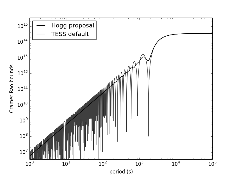
Recently, in conversations with Angus and Foreman-Mackey, I got interested in the asteroseismology angle on this: Could we do much better on asteroseismology by varying exposure times? I came up with a Cramér–Rao-bound formalism for thinking about this and started to code it up. It looks like a survey with (slightly) randomized exposure times vastly outperforms a survey with uniform exposure times on many fronts. Here's a plot from the first stab at this:


2015-04-17

Phil Marshall

Phil Marshall showed up today to give the astrophysics seminar. He also attended the CampHogg group meeting. In his seminar, he talked about finding and exploiting strong gravitational lenses in large sky surveys to make precise (and, importantly, accurate) inferences about the expansion history (or redshift—distance relation). He showed that when you are concerned that you might be affected by severe systematics, the best approach is to make your model much more flexible but then learn the relationships among the new nuisance parameters that make the much more flexible model nonetheless still informative. This requires hierarchical inference, which both Marshall and I have been pushing on the community for some years now.

In group meeting, he had the group members talk about the things they are most excited about. Among other things, this got Angus talking about periodograms with much better noise models under the hood and it got Foreman-Mackey talking about linear algebra tricks that might change our lives. Huppenkothen blew Marshall away with her example light-curves from GRS 1915. Marshall himself said he was excited about building a full three-dimensional model of all the mass density inside the Hubble volume, using both weak lensing and large-scale structure simultaneously. He has some ideas about baby steps that might make first projects tractable in the short run.

2015-04-16

recap

The only real research I did today was a recap of projects with Foreman-Mackey as he prepares to complete his thesis. There are a lot of projects open, and there is some decision-making about what ought to be highest priority.

2015-04-15

tracking the sky, spectroscopically

At group meeting today, Blanton spoke at length about telluric corrections and sky subtraction in the various spectroscopic surveys that make up SDSS-IV. His feeling is that the number of sky and telluric-standard fibers assigned in the surveys might not be optimal given the variability of the relevant systematics. He enlisted our help in analyzing that situation. In particular, what model complexity does the data support? And, given that model complexity, what is the best sampling of the focal plane with telluric standards (and sky fibers)? I agreed to write down some ideas for the SDSS-IV mailing lists.

2015-04-14

#astrohackny, week N+1

The day started at #astrohackny with Foreman-Mackey and I arguing about convolutions of Gaussians. The question is: Consider a model (probability of the data given parameters) with two (linear) parameters of importance and 150 (linear) nuisance parameters. There is a very weak Gaussian prior on the nuisance parameters. How to write down the marginalized likelihood such that you only have to do a 2x2 least squares, not a 152x152 least squares? I had a very strong intuition about the answer but no solid argument. Very late at night I demonstrated that my intuition is correct, by the method of experimental coding. Not very satisfying, but my abilities to complete squares with high-dimensional linear operators are not strong!

Taisiya Kopytova (MPIA) is visiting NYU for a couple of months, to work on characterizing directly imaged extra-solar planets. We discussed the simultaneous fitting of photometry and spectroscopy, one of my favorite subjects! I, of course, recommended modeling the calibration (or, equivalently, continuum-normalization) issues simultaneously with the parameter estimation. We also discussed interpolation (of the model grid) and MCMC sampling and the likelihood function.

At Pizza Lunch at Columbia, Chiara Mingarelli (Caltech) talked about the Pulsar Timing Array and its project to detect the stochastic background of gravitational waves. The beautiful thing about the experiment is that it detects the motion of the Earth relative to the pulsars, not the individual motions of the pulsars, and it does so using time correlations in timing residuals as a function of angle between the pulsars. The assumption is that the ball of pulsars is far larger than the relevant wavelengths, and that different pulsars are causally unconnected in time. Interesting to think about the "multiple hypotheses" aspects of this with finite data.

2015-04-13

vary all the exposure times!

Ruth Angus showed up for a few days, and we talked out the first steps to make an argument for taking time-series data with variable exposure times. We all know that non-uniform spacing of data helps with frequency recovery in time series; our new intuition is that non-uniform exposure time will help as well, especially for very high frequencies (short periods). We are setting up tests now with Kepler data but an eye to challenging the TESS mission to biting a big, scary bullet.

After complaining for the millionth time about PCA (and my loyal reader—who turns out to be Todd Small at The Climate Corporation—knows I love to hate on the PCA), Foreman-Mackey and I finally decided to fire up the robust PCA or PCP method from compressed sensing (not the badly-re-named "robust PCA" in the astronomy literature). The fundamental paper is Candès et al; the method has no free parameters, and the paper includes ridiculously simple pseudo-code. It looks like it absolutely rocks, and obviates all masking or interpolation of missing or bad data!

At lunch, Gabriele Veneziano (Paris, NYU) spoke about graviton–graviton interactions and causality constraints. Question that came up in the talk: If a particle suffers a negative time delay (like the opposite of a gravitational time delay), can you necessarily therefore build a time machine? That's something to dine out on.

2015-04-09

The Climate Corporation

I spent a bit of today at The Climate Corporation, hosted by former astronomer Todd Small. He told me about things they work on, which include field-level predictions for farmers about rainfall and sunlight, precise prediction and instructions for irrigation and fertilization, and advice about crop density (distances between seeds). He said they get data feeds from Earth observing but also from soil testing and even the farm machinery itself (who knew: combine harvesters produce a data feed!). A modern piece of large-scale farm equipment is precisely located on its path by GPS, makes real-time decisions about planting or whatever it is doing, and produces valuable data. They even have a tractor simulator in the house for testing systems.

We talked for a bit about the challenging task of communicating with clients (farmers, in this case) about probabilistic information, such as measurement uncertainties and distributions over predictions. This is another motivation for developing an undergraduate data-science educational program: It doesn't matter what industry you are in, you will need to be able to understand and communicate about likelihoods and posterior probabilities. I gave an informal seminar to a part of the climate modeling team about our uses of Gaussian Processes in exoplanet discovery.

2015-04-08

Caltech for a day

[On a research break this week; hence the lack of posts.]

I spent the day at Caltech Astronomy, with a dense schedule! Judy Cohen and I talked about RR Lyrae she is finding in the Milky Way halo and the challenge of getting a completeness function for statistical inferences. Pete Mao described to me the fiber positioners they are building for the Prime Focus Spectrograph multi-object spectrograph for Subaru. They have 50 seconds to get 2500 actuators in place (to a tolerance of 10-ish microns). Leslie Rogers and Ellen Price told me about Price's senior-thesis project to work out the composition constraints on short-period planets from tidal stress and the requirement that they not break up or mass-transfer. I was surprised to learn that there are some planets so close in that the tidal constraints rule out a range of compositions.

Nick Konidaris showed me new spectrographs being built in the high bay, and we talked about choices for spectral resolution. Adi Zitrin showed me amazing image of massive galaxy clusters he is using as telescopes to magnify very high-redshift galaxies; he has amazing examples, and also some nice techniques for building mass models. He does a great job of explaining arc multiplicity and morphology.

At lunch, students Rebecca Jensen-Clem and Michael Bottom told me about projects in high-contrast imaging, and Allison Strom and Sirio Belli told me about measuring the physical properties of galaxies in the redshift range 2 to 3. I tried to pitch my data-driven approaches at them: In the former area you might think about learning the actuator commands given the wavefront data directly from an optimization (with, presumably, the quality of the science image encapsulated in the objective function). In the latter, you might think about making a graph of galaxy spectra, where galaxies are joined by edges in the graph if their spectra are similar under any (reasonable) assumption about dust extinction. The students were (rightly) suspicious about both options!

Adam Miller and I discussed correct uses of machine learning in astronomy (since he is a great practitioner), and I once again pitched at him the possibility that we could try to replace their random-forest classifier in the time domain with a generative model of all stellar variable types. It would be hard, but exceedingly satisfying to do that. We discussed training-set imbalance and some clever ideas he has about combating it.

I asked Heather Knutson about how to get our (new) single transits we are finding in Kepler followed up with radial-velocity spectrographs. She made a great point about our future population inferences: Anything we infer from single transits makes a prediction for radial-velocity surveys and we should try to encourage the radial-velocity groups to confirm or deny in parallel. I discussed cadence and exposure-time issues for the Zwicky Transient Factory with Eric Bellm and visualization and interface for the LSST data with George Helou. I gave the Astrophysics Colloquium there about The Cannon and data-driven models (by my definition) and the day ended with a great dinner with Tom Soifer, Chuck Steidel, George Djorgovski, and Judy Cohen. It was a great trip!

2015-04-02

cosmology, now with less approximation; RNADE

In the morning, Mike O'Neil (NYU), Iain Murray (Edinburgh), Malz, Vakili, and I met for coffee to talk cosmology and cosmological inference. We discussed the linear algebra of making full (non-approximate) likelihood calls for cosmic background inference, which includes determinant and solve calls for enormous (dense) matrices. A few days ago, Wandelt made the (perhaps obscure) comment to me that he did his Gibbs sampling in the CMB to avoid making determinant calls. I finally understood this: The determinant is big and expensive in part because it is like an integral or marginalization over the nuisance parameters (which are the initial conditions or phases). If you can compute the determinant, you get something you can think of as being a marginalized likelihood function. The Gibbs sampling is part of a system that does posterior sampling, so it does the marginalization but doesn't return the amplitude of the likelihood function. If you need a marginalized likelihood function, you can't do it with the Gibbs sampling. Murray once again made the simple point that the posterior (for the cosmological parameters) will in general be much easier to compute and represent than the likelihood function (the probability of the data given the cosmological parameters) because the former is a much smaller-dimensional thing. That's a deep point!

That deep point played also into his talk in the afternoon about his RNADE method (and code) to use deep learning to represent very complex densities, or estimate a density given a sampling. One of his application areas is a project to obtain posterior constraints on the mass of the Milky Way given (as data) the properties of the Magellanic Clouds. The theory in this case is represented by a large number of numerical simulations, but Murray wants a continuous density to do inference. RNADE is really impressive technology.

2015-04-01

challenging inferences

Group meeting featured discussion from our two distinguished visitors this week, Brendon Brewer (Auckland) and Iain Murray (Edinburgh). Brewer described how he and Foreman-Mackey intend to re-do some exoplanet populations inference with something that he calls "joint-space sampling" and in the context of what you might call "likelihood-free inference" (although Brewer objects to even that label) or "approximate Bayesian computation" (a label I despise, because aren't all Bayesian computations approximate?).

The idea is that we have the counts of transiting systems with 0, 1, 2, or etc transiting planets. What is the true distribution of planetary system multiplicities implied by those counts? Brewer calls it joint-space sampling because to answer this question requires sampling in the population parameters, and all the parameters of all the individual systems. The result of the posterior inference, of course, depends on everything we assume about the systems (radius and period distributions, detectability, and so on). One point we discussed is what is lost or gained by restricting the data: In principle we should always use all the data, as opposed to just the summary statistics (the counts of systems). That said, the approach of Brewer and Foreman-Mackey is going to be fully principled, subject to the (strange) constraint that all you get (as data) are the counts.

Murray followed this up by suggesting a change to the ABC or LFI methods we usually use. Usually you do adaptive sampling from the prior, and reject samples that don't reproduce the data (accurately enough). But since you did lots of data simulations, you could just learn the conditional probability of the parameters given the data, and evaluate it at the value of the data you have. In general (his point is), you can learn these conditional probabilities with deep learning (as his RNADE code and method does routinely).

Murray also told us about a project with Huppenkothen and Brewer to make a hierarchical generalization of our Magnetron project published here. In this, they hope to hierarchically infer the properties of all bursts (and the mixture components or words that make them up). The challenge is to take the individual-burst inferences and combine them subsequently. That's a common problem here at CampHogg; the art is deciding where to "split" the problem into separate inferences, and how to preserve enough density of samples (or whatever) to pass on to the data-combination stage.

This was followed by Malz telling us about his project to infer the redshift density of galaxies given noisy photometric-redshift measurements, only just started. We realized in the conversation that we should think about multiple representations for surveys to output probabilistic redshift information, including quantile lists, which are fixed-length representations of pdfs. As I was saying that we need likelihoods but most surveys produce posteriors, Murray pointed out that in general posteriors are much easier to produce and represent (very true) so we should really think about how we can work with them. I agree completely.